9.6 Collinearity Equation

9.6 Collinearity Equation

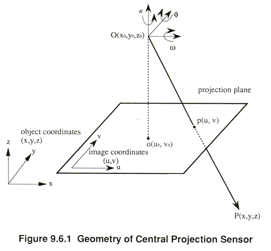
The Collinearity equation is a physical model representing the geometry between a sensor (projection center), the ground coordinates of an object and the image coordinates, while the coordinate transformation technique as mentioned in 9.5 can be considered as a black box type of correction. The collinearity equation gives the geometry of a bundle of rays connecting the projection center of a sensor, an image point and an object on the ground, as shown in Figure 9.6.1.

For convenience, an optical camera system is described to illustrate the principle. Let the projection center or lens be 0 (X0, Y0, Z0), with rotation angles , , around X, Y and Z axis respectively (roll, pitch and yaw angles), the image coordinates be p (x,y) and the ground coordinates be P(X,Y, Z). The collinearity equation is given as follows-

where f: focal length of lens, and a1 to a9 are given by the following matrix relationship.

In the case of a camera, the previous formula includes six unknown parameters (X0,Y0,Z0 ; , , ) which can be determined with the use of more than three ground control points (Xi,Yi; Xi,Yi,Zi). The collinearity equation can be inversed as follows-

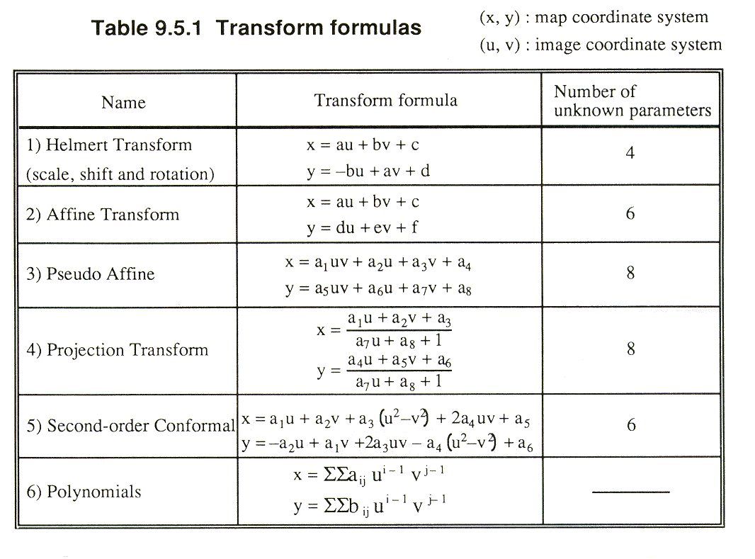
In the case of a flat plane (Z: constant), the formula coincides with the two dimensional projection as listed in Table 9.5.1. The geometry of an optical mechanical scanner and a CCD linear array sensor is a little different from the one of a frame camera. Only the cross track direction is a central projection similar to a frame camera, while along track direction is almost parallel (y=0) with a slight variation of orbit and attitude, as a function of time or line number, of not more than a third order as follows.

X0 = X0(l) = X0 + X1 l+ X2 l + X3 l
Y0 = Y0(l) = Y0 + Y1 l+ Y2 l + Y3 l
Z0 = Z0(l) = Z0 + Z1 l+ Z2 l + Z3 l
0 = 0(l) = 0 + 1 l+ 2 l + 3 l
0 = 0(l) = 0 + 1 l+ 2 l + 3 l
0 = 0(l) = 0 + 1 l+ 2 l + 3 l
, where l is line number.