
Pohang Earthquake (15 Nov 2017 Mw 5.4) observed by Sentinel-1A/B SAR Interferometry
Co-seismic Descending DInSAR (looking from east to west)
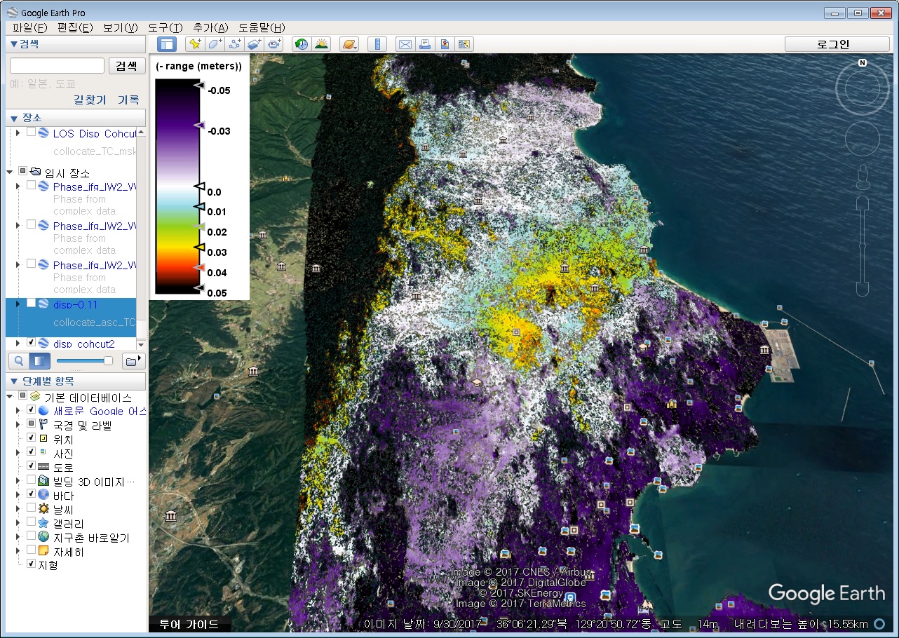
Figure 1. DInSAR Image. One cycle of RGB means 2.8 cm increase of range. Sentinel-1B was descending and right-looking.

Figure 2. LOS (Line Of Sight) displacement map. Positive values indicate uprising/easting of the land surface while negative values are subsidence/westing.

Figure 3. A zoomed image of Fig. 2 near the epicenter. Red to yellow patches (>3cm uprising/easting) coincide with the mountains while cyan to green patches (<2 cm) are rice fields on alluvial plain after harvest. Beside a DEM error, one possible explanation is that alluvial plain could not be elastically restored fully due to the compaction thus subsidence after liquefaction (discussed with T. S. Kang at PKNU). Several cases of the soil subsidence around buildings have been confirmed by field investigation (J. H. Park and S. R. Lee at KIGAM). Slight change of displacement within the alluvial plain, especially near the mountain, might imply the varying depth of the alluvial plain (discussed with J. H. Park at KIGAM).

Figure 4. Preliminary interpretation of the focal mechanism (discussed with T. S. Kang at PKNU, J. Rhie at SNU, and H. K. Lee at KNU). The location of the aftershock hypocenters has been modified slightly northwest following the discussion with J. H. Park at KIGAM.

Figure 5. Static slip distribution model for the Pohang earthquake obtained by inverting the InSAR data (modeled by S. G. Song at KIGAM).
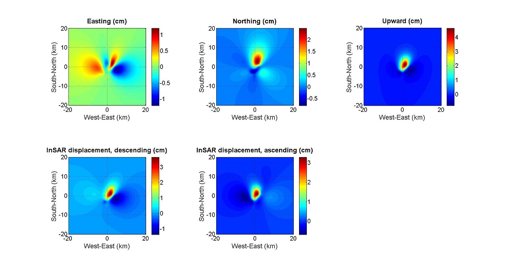
Figure 6. Three dimensional surface displacement map calculated from the static slip distribution model in Fig. 5 (provided by S. G. Song at KIGAM). Note the lower-left image is the predicted descending InSAR displacement with LOS=(0.6329, -0.1126, 0.7660) while the lower-right is the predicted ascending InSAR displacement with LOS=(-0.6262, -0.1451, 0.7660).
Google Earth KMZ
The LOS (Line of Sight) unit vector of a right-looking radar in (x, y, z)=(E, N, UP) coordinates is given by
LOS (from surface to satellite)= ( - sin a * cos b, sin a * sin b, cos a ),
where a: local incidence angle between z-axis and LOS,
b: satellite heading projected on the x-y plane measured clockwise from N.
For example,
Descending, right looking : if a = 40 deg and b = 190.0847114240353 deg , then LOS = ( 0.6329, -0.1126, 0.7660 ).
Ascending, right looking : if a = 41 deg and b = -13.04524393024839 deg, then LOS = (-0.6391, -0.1481, 0.7547 ).
SAR Data: Sentinel Data Hub
S1B_IW_SLC__1SDV_20171104T212321_20171104T212347_008137_00E617_DAB0.zip
S1B_IW_SLC__1SDV_20171104T212345_20171104T212420_008137_00E617_33CD.zip
S1B_IW_SLC__1SDV_20171116T212320_20171116T212347_008312_00EB57_E878.zip
S1B_IW_SLC__1SDV_20171116T212345_20171116T212419_008312_00EB57_910A.zip
Software and Data Processing
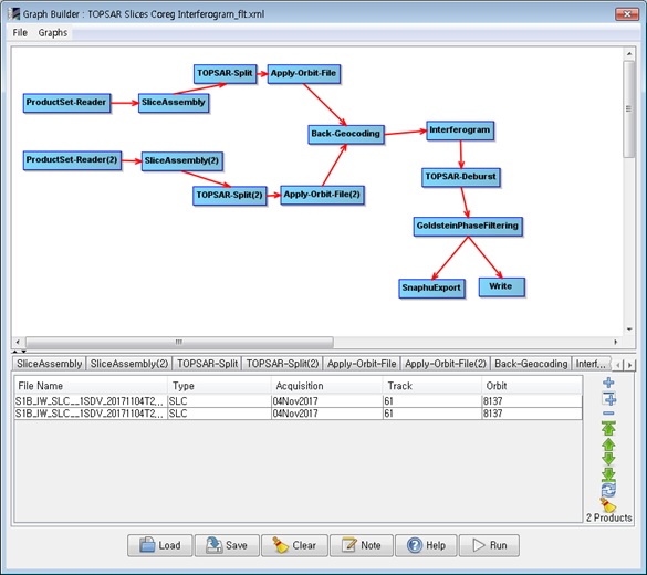
Supplementary Figure 1. SNAP Graph Builder with SliceAssembly.
SNAP Graph Builder:
Sentinel-1B Descending Right-looking
04Nov2017 – 16Nov2017 21:23:21 UST
Slice Assembly: VV
TOPSAR-Split: IW2, 6-15 bursts out of 20
Back-Geocoding: SRTM 1Sec HGT (Auto Download)
Interferogram: Subtract flat-earth phase and topographic phase
CPU time < 1hr with Intel i7 / 32GB Memory
SNAP-Snahpu subsequent processing:
Mask Sea Area for Snaphu
Raster -> Masks -> Land/Sea Mask: Mask out the sea, Use SRTM 3sec
Image right click -> Spatial subset from view (optional)
File -> Export -> Beam-DIMAP (if subset)
Snaphu Export
Radar -> Interferometric -> Unwrapping -> Snaphu Export
Run snaphu in VMWare Ubuntu 14.04
Execute command in snaphu.conf file.
Snaphu Import
Phase to Displacement
Radar -> Interferometric -> Products -> Phase to Displacement
Collocate the displacement into the interferogram
Raster -> Geometric Operations -> Collocation
Band Math: If coh < 0.3 then NaN else disp
Terrain Geocoding
Radar -> Geometric -> Terrain Correction -> Range-Doppler Terrain Correction
Export to Google Earth KMZ
Colour Manipulation
Image right click -> Spatial Subset from view : (<20MB)
Image right click -> Export View as Google Earth KMZ
IRIS Earthquake Resources
Post-seismic Descending DInSAR Analysis


Figure 7. Post-seismic DInSAR and LOS displacement map (Sentinel-1B, descending right looking. 16-28 Nov 2017). No significant post-seismic displacements are observed. Most signals are considered as of atmospheric perturbation or soil moisture change during the 12 days after the main shock on 15 Nov 2017. Here are the KMZ files of DInSAR, LOS displacement, and LOS displacement with coherence cut of 0.2.
Co-seismic Ascending DInSAR (looking from west to east)

(a) DInSAR (IW2)

(b) A zoomed up image of (a) DInSAR near the epicenter
(c) LOS displacement map near the epicenter. Ascending, right looking : if a = 41 deg and b = -13.04524393024839 deg, then LOS = (-0.6391, -0.1481, 0.7547 ).
Figure 8. Co-seismic DInSAR and LOS displacement map obtained from Sentinel-1A, ascending right looking, 10 Nov - 4 Dec 2017 InSAR pair. Similar displacement patterns (~3 cm) are observed near the epicenter when compared with the descending orbit, although very low coherence poses difficulties in phase unwrapping or interpretation due to the 24-days of temporal decorrelation, atmospheric delay, and/or soil moisture change. Here are the KMZ files of DInSAR, LOS displacement, LOS displacement > Coherence 0.2, and LOS displacement > Coherence 0.3. To extract data you can download the black(-0.1 m) and white(0.1 m) KMZ files of LOS displacement, LOS displacement > Coherence 0.2, and LOS displacement > Coherence 0.3. You may also find that a coherence image in black(0) and white(1) and local incidence angle in black (40 deg) and white(42 deg) KMZ files are useful for slip displacement modeling.
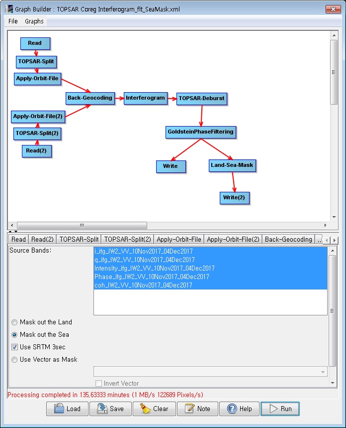
Supplementary Figure 2. SNAP Graph Builder with Land-Sea-Mask (without SliceAssembly).
All rights reserved by Prof. Hoonyol Lee, Division of Geology and Geophysics, Kangwon National University.
Last updated on 2017/12/11 월요일 09:42:11 +0900